Chapter 18

Performance

Performance means at least two things in computing:

Application development speed
Execution speed

Python addresses the first issue with clear syntax and extensive power and flexibility. As to the second issue, Python has a reputation for slowness.

Is It Too Slow?

Computer programming projects have a long history of premature optimization: optimizing before any measurement shows where the time goes. Often people decide ahead of time, based on biases, that runtime performance will be insufficient. They then build elaborate, expensive designs that solve nonexistent problems.

Python can be surprising. A program coded in the most straightforward way, without concern for performance, can often run fast enough for your needs. Do not automatically assume that a simply written program will be too slow. Try it out first. It might be fine.

The opposite assumption fails just as often: a program that works in the small may not scale. A run over a hundred records says nothing about a million, because costs grow at different rates. An algorithm that revisits its data looks instant at one size and takes hours at another, and every layer of abstraction hides costs (a copy per call, a query behind an attribute) that only a realistic load reveals. So “try it out” means try it at the size you expect in production, not at the size that is convenient to type.

If it is too slow, try the simplest remedy first. That might be enough, and if it is, you save time and money.

The rest of this chapter works through performance problems, starting with the simplest techniques and growing successively more complex.

Try a Faster Platform

The cheapest platform change is a newer CPython. 3.11 alone measured 1.25x faster than 3.10 across the pyperformance suite, a range of 10-60% depending on the workload, and later releases have continued that work. Moving a project forward two or three releases costs a test run rather than a rewrite. A speedup that needs neither new code nor new hardware is rare.

Two more speedups need no new code: the tail-calling interpreter, and the experimental just-in-time compiler inside CPython, the subjects of the next two sections.

Alternative interpreters for Python exist, notably PyPy, which claims about a 3x speedup on average. PyPy typically trails CPython’s newest language version, so confirm it supports the features and third-party packages you need.

For a parallel, CPU-bound workload, the free-threaded build (The GIL and Free Threading) is the largest platform-level speedup available in 3.15, since it removes the lock that otherwise serializes Python bytecode across threads.

How much does a hardware upgrade cost compared to paying programmers to solve the performance problem? If it’s noticeably less, buying new hardware might be a quick win.

The Tail-Calling Interpreter

The first of those speedups has no switch. Since 3.14, CPython can be built so that each bytecode instruction is a small C function that ends by calling the function for the next instruction, in place of one large C switch that dispatches every instruction. The C compiler turns each of those calls into a jump, and the loop that runs Python bytecode gets faster. The tail call is in C, inside the interpreter. It is unrelated to tail-call optimization of Python functions, which CPython does not do, as Recursion notes.

Nothing in your program changes, and nothing in your program can tell. No sys function reports it, and the documentation calls it an internal detail. The build decides. The python.org Windows 64-bit binaries for 3.15 use it, as do the python-build-standalone 3.15 builds that uv installs, including the interpreter that runs this book’s listings. A source build needs --with-tail-call-interp and a compiler with the preserve_none calling convention: Clang 19 or newer, or Visual Studio 2026.

The payoff is again a percentage, and a larger one than the JIT’s. On Windows x86-64, 3.15 measures 15-20% faster on the pyperformance geometric mean than the same source built with the switch, with individual programs from 14% to 40%. The 3.14 figure, with Clang 19, is 3-5%.¹ The two speedups stack. The JIT compiles the hot paths, the tail-calling interpreter runs everything else faster, and the macOS figure in the next section is measured on top of this one.

The CPython JIT

CPython includes an experimental just-in-time compiler. PEP 744 added it in 3.13, and 3.15 rebuilt much of it. The JIT watches the bytecode a program executes, and once a path runs often enough, it compiles that path to machine code. You change nothing. The same file runs, and the interpreter stops re-interpreting its busiest paths.

Three switches stand between your program and that machine code:

The interpreter must be built with the JIT, through the --enable-experimental-jit configuration option. Building it needs LLVM. Running the result does not.
The process must enable it, through the PYTHON_JIT environment variable.
The code must get hot. A script that runs briefly and exits never reaches the threshold, so it pays the compiler’s warm-up and collects nothing.

Since 3.14, the official python.org Windows and macOS binaries use --enable-experimental-jit=yes-off, which compiles the JIT in and leaves it switched off, so PYTHON_JIT=1 turns it on. Plain yes builds start with the JIT running, and there PYTHON_JIT=0 turns it off. Other distributions decide for themselves, so the first question is not “is the JIT on?” but “which build am I running?” sys._jit answers it:

# jit_status.py
import sys

def jit_state() -> str:
    if not sys._jit.is_available():
        return "no JIT in this build"
    if not sys._jit.is_enabled():
        return "JIT built in, switched off"
    return "JIT enabled"

print(jit_state())
#: no JIT in this build

is_enabled() implies is_available(), so testing is_available() first and is_enabled() second names the three states a build can be in.

Most listings in this book print the same line on every machine. This one changes with your interpreter. The book’s build has no JIT compiled in, so it prints the first line. A python.org binary prints the second until you set PYTHON_JIT=1.

A third function, sys._jit.is_active(), reports whether the frame that called it is running compiled code. The documentation warns against branching on its result, since a tracing compiler can give different answers to the same call.

The payoff is a percentage, not a multiple. On the pyperformance suite, 3.15 measures 8-9% faster on x86-64 Linux against the standard optimized build, and 12-13% faster on AArch64 macOS against the tail-calling interpreter. Those are geometric means over dozens of benchmarks, and the What’s New marks them as not yet final. The report sets aside one microbenchmark, unpack_sequence, and the rest range from roughly 15% slower to more than twice as fast, so the mean predicts your program poorly. Measuring your own program costs two runs: time the workload with PYTHON_JIT set to 1 and to 0, and change nothing else.

Numba’s @njit, later in this chapter, is also a just-in-time compiler, and the two make opposite trades. The CPython JIT asks nothing of you, applies to whatever code turns out to be hot, and pays in single-digit percentages. @njit applies only to numeric functions, costs a decorator and a compilation pause on the first call, and pays in multiples. Neither one rescues a quadratic algorithm.

PEP 836 sets the bar the JIT must clear: 5% over the interpreter alone for 3.16, then 20% for the JIT combined with free threading by 3.17. The PEP calls that the minimum for continuing to develop the JIT inside CPython, and even then, turning it on by default would need separate approval from the release manager.

Profilers

A profiler looks for the slow spots in your code, so you know where to focus. You may think you “have a pretty good idea where the slowdown is,” but programmers turn out to be bad at guessing. A profiler tells you for sure, preventing wasted time.

The standard library includes two. The first is the classic cProfile, a deterministic tracing profiler that arrived in 2006 and records every function call and return. The second, new in Python 3.15, is a sampling profiler. cProfile’s numbers are exact, but the instrumentation slows the program, sometimes enough to distort the behavior you are measuring. Here’s how you run cProfile on my_program.py:

uv run python -m cProfile -s cumulative my_program.py

The report is a table, one row per function. This one profiles a small script, prof_demo.py, built with one obvious hot spot and one function called too many times:

# prof_demo.py
def helper() -> int:
    return sum(i * i for i in range(10_000))

def slow() -> None:
    total = 0
    for i in range(2_000_000):
        total += i
    helper()

if __name__ == "__main__":
    slow()

Running it under the profiler prints a table like this one (the exact times vary by machine, so treat these as one sample run, not a value the book asserts):

$ uv run python -m cProfile -s cumulative prof_demo.py
   ncalls  tottime  percall  cumtime  percall filename:lineno(function)
        1    0.000    0.000    0.077    0.077 {built-in method builtins.exec}
        1    0.000    0.000    0.077    0.077 prof_demo.py:1(<module>)
        1    0.074    0.074    0.077    0.077 prof_demo.py:5(slow)
        1    0.000    0.000    0.003    0.003 prof_demo.py:2(helper)
        1    0.002    0.002    0.003    0.003 {built-in method builtins.sum}
    10001    0.001    0.000    0.001    0.000 prof_demo.py:3(<genexpr>)

tottime is the time spent inside that function alone. cumtime adds the time spent in everything it called. Sorting by cumtime puts exec and <module> on top, which tells you nothing: they call everything, so they contain everything. Scan down to the first row where tottime is large: here, slow(). That is the function to attack, since its own loop, not anything it calls, burns most of the time. ncalls decides how to attack it. slow() spends most of the total in a single call, so it needs a better algorithm. <genexpr>’s ten thousand calls show helper() paying per-element overhead, where fewer calls would help more than a faster body.

Python 3.15 gathers the profilers into a single profiling package (PEP 799). The deterministic tracing profiler becomes profiling.tracing, and cProfile remains an alias. 3.15 deprecates the old pure-Python profile module, and 3.17 removes it, so use profiling.tracing or cProfile for tracing. The sampling profiler is profiling.sampling. Instead of tracing every call, it takes periodic snapshots of the call stack, so the overhead is near zero and the program runs at full speed while you watch. You invoke it like this:

uv run python -m profiling.sampling run my_program.py

The new profiler can also attach to a process that is already running, using the process ID. Attaching makes it the tool for a slowdown you can only reproduce live:

uv run python -m profiling.sampling attach 12345

Either form ends with a table of hot functions ranked by sample count.

Beyond the standard library, Scalene separates Python time from native time and profiles memory line by line.

Measuring One Function with `sys.monitoring`

A profiler answers a broad question about the whole program. Sometimes you have a narrow one: how many times does this function run during a request, and does that branch run at all? A counter added to the function changes the code you are studying, and a full profiler costs more than the answer is worth.

sys.monitoring (PEP 669) is the interpreter’s own instrumentation mechanism, the one profilers and debuggers now use. You claim a tool identifier, register a callback for an event, and say which code the event applies to. Registering nothing costs nothing: the interpreter specializes the bytecode that has no callback attached, so unmonitored code runs at full speed. sys.settrace(), by contrast, slows every Python function in the process, since its trace function runs on each call and then on each line:

# monitoring_counts.py
import sys
from collections import Counter
from types import CodeType
from typing import Final

monitoring = sys.monitoring
TOOL: Final[int] = monitoring.PROFILER_ID
PY_START: Final[int] = monitoring.events.PY_START
NO_EVENTS: Final[int] = monitoring.events.NO_EVENTS
counts: Counter[str] = Counter()

def on_start(code: CodeType, offset: int) -> None:
    counts[code.co_name] += 1

def fib(n: int) -> int:
    return n if n < 2 else fib(n - 1) + fib(n - 2)

def square(n: int) -> int:
    return n * n

monitoring.use_tool_id(TOOL, "call counter")
monitoring.register_callback(TOOL, PY_START, on_start)
monitoring.set_local_events(TOOL, fib.__code__, PY_START)
print(fib(10), square(4))
#: 55 16
monitoring.set_local_events(TOOL, fib.__code__, NO_EVENTS)
monitoring.free_tool_id(TOOL)
print(counts)
#: Counter({'fib': 177})

fib() and square() stay untouched. The counting lives outside them, in on_start(), which the interpreter calls each time a monitored Python function begins. set_local_events() is the narrow instrument: it attaches the event to one code object, and that is why square() is absent from the count even though it ran. The event does not spread to whatever that code calls, so a helper that fib() invokes would go uncounted as well. The global form is set_events(), which fires for every Python function in the process, and that is where the two differ in cost. When one function is the question, set_events() collects data you discard and slows the run you are measuring.

set_local_events() with NO_EVENTS detaches, and free_tool_id() releases the identifier. The identifiers are a shared resource: PROFILER_ID, DEBUGGER_ID, and COVERAGE_ID carry the names of their intended users. Claiming one that another tool already holds raises a ValueError, so two profilers never fight silently over the same callbacks.

For an answer you need once rather than continuously, the callback can turn its own event off:

# monitoring_coverage.py
import sys
from collections import Counter
from types import CodeType
from typing import Final

monitoring = sys.monitoring
TOOL: Final[int] = monitoring.COVERAGE_ID
PY_START: Final[int] = monitoring.events.PY_START
NO_EVENTS: Final[int] = monitoring.events.NO_EVENTS
calls: Counter[str] = Counter()

def on_start(code: CodeType, offset: int) -> object:
    calls[code.co_name] += 1
    return monitoring.DISABLE

def used(n: int) -> int:
    return n + 1

def unused(n: int) -> int:
    return n - 1

monitoring.use_tool_id(TOOL, "coverage")
monitoring.register_callback(TOOL, PY_START, on_start)
monitoring.set_events(TOOL, PY_START)
print(sum(used(n) for n in range(1000)))
#: 500500
monitoring.set_events(TOOL, NO_EVENTS)
monitoring.free_tool_id(TOOL)
print(calls["used"], calls["unused"])
#: 1 0

Returning monitoring.DISABLE tells the interpreter to stop reporting this event at this location until someone calls restart_events(). used() ran a thousand times and the callback ran once. That makes coverage measurement affordable: the question is “was this reached,” so the second answer is worthless, and after the first hit the monitored code returns to full speed.

The trade against a profiler is the usual one. A profiler gives you a ranked table with no code to write. sys.monitoring gives you one number about one function, and that is the better tool when you know which function matters and the profiler’s overhead would change the answer.

Benchmark Alternatives with `timeit`

A profiler tells you where the time goes. Once you discover a hot spot, timeit tells you which rewrite wins. It runs a small snippet many times and reports the total, insulating the measurement from startup cost and clock granularity.

Timings differ from machine to machine, so the following example prints a comparison instead of raw numbers. The numbers are one flag away: run any measured listing in this book with --numbers to see what your machine did (Numbers on Your Machine). A list tests membership by scanning. target in as_list walks the list from the start, comparing each element until it finds a match or reaches the end. A set tests membership through hashing. target in as_set computes a hash of target and jumps to the bucket that value occupies. Scanning gets slower as the list grows. Hashing stays fast no matter how many elements the set holds:

# membership.py
import timeit
from benchmark import report

n = 100_000
as_list = list(range(n))
as_set = set(as_list)
target = n - 1  # Worst case: the last element in the list

t_list = timeit.timeit(
    lambda: target in as_list, number=100
)
t_set = timeit.timeit(lambda: target in as_set, number=100)
report(list_scan=t_list, set_lookup=t_set,
       ratio=t_list / t_set)
print(f"set at least 100x faster: {t_set * 100 < t_list}")
#: set at least 100x faster: True

timeit.timeit() calls its first argument repeatedly and returns the total elapsed time in seconds for every call combined, not the time for one call. That first argument is a lambda here rather than a string of code, since a lambda can close over target, as_list, and as_set directly, with no separate setup argument needed to build them. number sets how many times timeit calls the lambda, 100 in this case. Leaving number out defaults to a million calls, which suits a microsecond snippet and is a long wait for anything slower, so always set it for a function you have not timed before. One machine measured the set at about 14,000 times faster than the list scan.

A single measurement includes whatever else the machine was doing. timeit.repeat(f, number=100, repeat=5) returns a list of five such totals, and the smallest of them is the run with the least interference. Report min(...), not the mean: a slow run means something stole the CPU, so averaging folds that theft into your answer, while the fastest run is the closest you got to measuring only your code.

A single lookup costs little either way. A million lookups is the difference between instant and minutes. timeit also has a command-line form for one-off questions:

uv run python -m timeit -s "s = set(range(100_000))" "99_999 in s"

Benchmark with data shaped like production data. A list of ten elements can beat a set, and an optimization tuned to toy input can behave badly in production.

timeit also turns the garbage collector off while it measures, so its runs stay repeatable. For a benchmark that allocates heavily, that hides a cost production pays, so pass setup="gc.enable()" when collection pauses are part of what you are comparing.

Numbers on Your Machine

Every measured listing in this book prints a threshold rather than a measurement, so the book’s output is the same on your machine as on mine. Each listing still takes its measurements, and one flag prints them:

# utils/benchmark.py
import sys
from typing import Final

NUMBERS: Final[bool] = "--numbers" in sys.argv

def report(**measured: float) -> None:
    # Print each measurement, but only under --numbers:
    if not (NUMBERS and measured):
        return
    width = max(len(name) for name in measured)
    for name, value in measured.items():
        if isinstance(value, int):
            shown = f"{value:,}"  # Byte counts stay whole
        else:
            shown = f"{value:,.6f}"
        print(f"  {name:<{width}} {shown}")

report() prints when the flag is present and stays silent otherwise, so the listing’s own output, the line the book shows, never changes. Running membership.py with the flag adds the measurements above it:

$ uv run python membership.py --numbers
  list_scan  0.041807
  set_lookup 0.000003
  ratio      13,935.560574
set at least 100x faster: True

The names are the keyword arguments at the call site, so each listing labels its own measurements. Your ratio differs from the one above; seeing your own number is the point of running it.

Write Idiomatic Python

The interpreter is a C program. A built-in like sum() runs its loop in C, so the more of your loop you hand to C, the less bytecode runs per element. The idiomatic version of a loop is usually also the fast one:

# builtin_sum.py
import timeit
from benchmark import report

numbers = list(range(100_000))

def hand_written() -> int:
    total = 0
    for n in numbers:
        total += n
    return total

assert hand_written() == sum(numbers)
t_loop = timeit.timeit(hand_written, number=50)
t_sum = timeit.timeit(lambda: sum(numbers), number=50)
report(hand_written=t_loop, builtin_sum=t_sum)
print(f"sum() at least twice as fast: {t_sum * 2 < t_loop}")
#: sum() at least twice as fast: True

One machine measured sum() at about five times faster than the hand-written loop.

Other examples:

String concatenation: "".join(parts) is faster than += in a loop (one linear pass instead of repeated reallocation).
A comprehension is faster than an append() loop, though the margin is now small (one bytecode appends the element, instead of an attribute lookup and a call). Write it for the readability. The speed is a rounding error.
The C-implemented standard library’s itertools, collections, and functools are faster than hand-rolled equivalents (Iterators tours the iterator algorithms).

As a last resort in a proven hot loop, hoist a repeated attribute or global lookup into a local, as in append = out.append. That is a micro-optimization, so let a measurement justify it:

# hoist_attribute_lookup.py
import timeit
from benchmark import report

n = 100_000

def with_attribute_lookup() -> list[int]:
    out: list[int] = []
    for i in range(n):
        out.append(i)
    return out

def with_hoisted_local() -> list[int]:
    out: list[int] = []
    append = out.append
    for i in range(n):
        append(i)
    return out

assert with_attribute_lookup() == with_hoisted_local()
t_attr = timeit.timeit(with_attribute_lookup, number=100)
t_local = timeit.timeit(with_hoisted_local, number=100)
report(attribute_lookup=t_attr, hoisted_local=t_local)
print(f"hoisting did not halve the time: "
      f"{t_local * 2 > t_attr}")
#: hoisting did not halve the time: True

Here the hoist does not pay off, and it can cost. out.append(i) compiles to a method load that pushes the function and its self separately, building no bound method. append = out.append builds one, and every call then goes through it. One machine measured the hoisted version five percent slower, another twenty. Measure it on your own machine before believing either direction. The threshold is deliberately loose. Timing noise on a busy machine easily reaches ten or twenty percent, so a claim about a small difference measures the machine’s mood. A hoist worth writing beats that margin without argument. The measurement proves the point because it catches a “classic” optimization that no longer works, just as readily as it catches one that does.

Choose Better Algorithms and Data Structures

The biggest speedups usually come from a better algorithm. Choosing an algorithm with lower Big-O complexity beats micro-optimizing a slow one. Often the better algorithm is a better container. Use a set or dict for membership and lookup instead of scanning a list. Use a deque (see Containers) when you add and remove at both ends.

Bisect

For data kept in sorted order, the bisect module finds the insertion point using binary search:

# bisect_search.py
import bisect
from typing import Final

CUTOFFS: Final[list[int]] = [60, 70, 80, 90]
LETTERS: Final[str] = "FDCBA"

scores = [60, 70, 75, 90]  # Must stay sorted
i = bisect.bisect(scores, 78)  # Where 78 goes
print(i)
#: 3
bisect.insort(scores, 78)  # Insert and keep it sorted
print(scores)
#: [60, 70, 75, 78, 90]

def grade(score: int) -> str:
    # Map a score to a letter through its cutoff boundaries:
    return LETTERS[bisect.bisect(CUTOFFS, score)]

print([grade(s) for s in (55, 65, 85, 95)])
#: ['F', 'D', 'B', 'A']

Because scores stays sorted, bisect locates a position in O(log n) instead of the O(n) scan a list needs. bisect() is an alias for bisect_right(), which returns the position after any elements equal to the target, while bisect_left() returns the position before them (insort() is likewise an alias for insort_right()). Either one answers “where does this go,” but when the target is already in the list, only bisect_left() returns its index, so a membership test must use it, as search_comparison.py does below. The speed is in the search alone: insort() still shifts everything after the insertion point. Under heavy insert traffic consider the heap below instead.

Comparison

That leaves three ways to answer the same membership question: scan a list, binary-search a sorted list with bisect, or hash straight to the answer with a set. Timing all three together shows the size of each step:

# search_comparison.py
import bisect
import timeit
from benchmark import report

n = 100_000
as_list = list(range(n))
as_set = set(as_list)
target = n // 2

def scan() -> bool:
    return target in as_list

def binary_search() -> bool:
    i = bisect.bisect_left(as_list, target)
    return i < len(as_list) and as_list[i] == target

def hashed() -> bool:
    return target in as_set

assert {scan(), binary_search(), hashed()} == {True}
t_scan = timeit.timeit(scan, number=1000)
t_search = timeit.timeit(binary_search, number=1000)
t_hashed = timeit.timeit(hashed, number=1000)
report(scan=t_scan, binary_search=t_search, hashed=t_hashed)
print(f"binary search at least 100x faster than scan: "
      f"{t_search * 100 < t_scan}")
#: binary search at least 100x faster than scan: True
print(f"hashing at least 3x faster than binary search: "
      f"{t_hashed * 3 < t_search}")
#: hashing at least 3x faster than binary search: True

The scan loses badly, since it walks roughly half the list before reaching target. bisect narrows that to a handful of comparisons, one per halving of the remaining range, and that is why the move from O(n) to O(log n) shows up here as orders of magnitude rather than a modest improvement. Hashing wins again over bisect, since it needs only one hash and one equality check no matter how large as_set grows. One machine measured bisect at about 2,000 times faster than the scan, and hashing at about five times faster than bisect.

Heap

When you repeatedly need the smallest or largest item, a heap keeps that item reachable in O(log n). The heapq module treats a list as a binary heap:

# heap_queue.py
import heapq

nums = [5, 1, 8, 3, 2]
heapq.heapify(nums)  # Rearrange into a min-heap in place
print(nums)
#: [1, 2, 8, 3, 5]
print(nums[0])  # The smallest stays at the front
#: 1
heapq.heappush(nums, 7)
print(nums)
#: [1, 2, 7, 3, 5, 8]
print(heapq.heappop(nums))  # Remove and return the smallest
#: 1
print(nums)
#: [2, 3, 7, 8, 5]
# Does not reorder the argument:
print(heapq.nsmallest(3, [5, 1, 8, 3, 2]))
#: [1, 2, 3]
print(heapq.nlargest(2, [5, 1, 8, 3, 2]))
#: [8, 5]

After heapify() the smallest element sits at index 0. nsmallest() and nlargest() answer top-N questions without heapifying the list first.

Through Python 3.13, heapq only built a min-heap. Getting a max-heap meant negating every value going in and out. Python 3.14 added _max variants (heapify_max(), heappush_max(), heappop_max(), and friends) that keep the largest item at index 0 instead, so the negation trick is no longer necessary:

# max_heap_queue.py
import heapq

max_nums = [5, 1, 8, 3, 2]
# Rearrange into a max-heap in place
heapq.heapify_max(max_nums)
print(max_nums)
#: [8, 3, 5, 1, 2]
print(max_nums[0])  # The largest stays at the front
#: 8
heapq.heappush_max(max_nums, 9)
print(max_nums)
#: [9, 3, 8, 1, 2, 5]
# Remove and return the largest
print(heapq.heappop_max(max_nums))
#: 9
print(max_nums)  # Heap ordering is maintained
#: [8, 3, 5, 1, 2]

Every operation mirrors its min-heap partner, with heapify_max() putting the largest element at index 0.

The output shows the list in the order the heap-management algorithm keeps it, which is not sorted order. Use the heap version of every operation. The list’s own pop(0) returns the smallest value the first time, but it also destroys the heap ordering, so a second pop(0) would return 6 while 4 is still in the list:

# heap_corruption.py
from heapq import heapify, nsmallest

heap = [10, 9, 8, 7, 6, 5, 4, 3]
heapify(heap)  # In-place
print(heap)
#: [3, 6, 4, 7, 10, 5, 8, 9]
print(heap.pop(0))  # Smallest
#: 3
print(heap)  # 'heap[0]' no longer smallest
#: [6, 4, 7, 10, 5, 8, 9]
print(nsmallest(len(heap), heap))  # True smallest
#: [4, 5, 6, 7, 8, 9, 10]
print(heap)  # Not reordered by nsmallest()
#: [6, 4, 7, 10, 5, 8, 9]

For a priority queue shared across threads, queue.PriorityQueue wraps the same heap in a lock. Concurrency shows it in use.

A heap answers a different question than a hash-based container. A set tells you whether a value is present in O(1), but it knows nothing about order, so finding the smallest values still means scanning or sorting every item. A heap keeps the smallest item at hand as you push and pop, so pulling it costs only O(log n) each time, no matter how many times you repeat it. The natural competitor for “give me the 100 smallest” is not a scan, but sorted(data)[:100], so that is what the heap needs to beat:

# heap_vs_hash.py
import heapq
import random
import timeit
from benchmark import report

n = 10_000
data = list(range(n))
random.seed(0)
random.shuffle(data)  # Neither side gets a free ride

def heap_min_extractions() -> list[int]:
    heap = data.copy()
    heapq.heapify(heap)
    return [heapq.heappop(heap) for _ in range(100)]

def sorted_min_extractions() -> list[int]:
    return sorted(data)[:100]

assert (heap_min_extractions()
        == sorted_min_extractions())
t_heap = min(timeit.repeat(
    heap_min_extractions, number=50, repeat=5
))
t_sorted = min(timeit.repeat(
    sorted_min_extractions, number=50, repeat=5
))
report(heap=t_heap, sorted_slice=t_sorted)
print(f"heap beats sorted() by 1.5x+ on shuffled "
      f"data: {t_heap * 1.5 < t_sorted}")
#: heap beats sorted() by 1.5x+ on shuffled data: True

sorted(data) orders every element up front, costing O(n log n) no matter how few items you then take. heapify() pays O(n) once, then each heappop() costs only O(log n), so the same 100 extractions cost roughly O(n + 100 log n), smaller than sorting whenever the fraction you extract stays small. One machine measured the heap at about 3 times faster here. The comparison only holds when the input order gives neither side an advantage. On descending data, the kind heap_corruption.py uses, Timsort detects the existing run and sorted() wins outright. A heap is not automatically the right choice. Measure with data shaped like production data. heapq.nsmallest(100, data), introduced above, answers this exact “top-N” question directly, and is the tool to use before hand-rolling either comparison here. The heap fits a different shape of problem: pushes and pops interleaved over time, with nothing to presort in advance. Re-sorting after every insertion would cost far more than one incremental heappush()/heappop() pair.

The immutable containers from Containers are not a speed upgrade. A frozenset looks up just as fast as a set, a frozendict behaves like a dict, and a tuple scans like a list. In CPython these share the same machinery. Choose immutability for correctness and safe sharing. Immutable values are hashable, so they can serve as dictionary keys and as arguments to the caches below.

Lazy Evaluation with Generators

A list-building pipeline materializes every intermediate result. A generator pipeline (Comprehensions) computes one item at a time, on demand, so memory use doesn’t grow with the size of the source, and the pipeline does no work past the point where the consumer stops. tracemalloc measures the difference:

# lazy_pipeline.py
import tracemalloc
from itertools import islice
from benchmark import report

n = 1_000_000

def eager_first_evens() -> list[int]:
    squares = [x * x for x in range(n)]
    evens = [s for s in squares if s % 2 == 0]
    return evens[:5]

def lazy_first_evens() -> list[int]:
    squares = (x * x for x in range(n))
    evens = (s for s in squares if s % 2 == 0)
    return list(islice(evens, 5))

tracemalloc.start()
eager = eager_first_evens()
_, eager_peak = tracemalloc.get_traced_memory()
tracemalloc.stop()

tracemalloc.start()
lazy = lazy_first_evens()
_, lazy_peak = tracemalloc.get_traced_memory()
tracemalloc.stop()

print(eager, eager == lazy)
#: [0, 4, 16, 36, 64] True
report(eager_peak_bytes=eager_peak,
       lazy_peak_bytes=lazy_peak)
print(f"lazy peak under 1% of eager: "
      f"{lazy_peak * 100 < eager_peak}")
#: lazy peak under 1% of eager: True

Both versions produce the same five numbers, but the eager one builds a million-element list and a half-million-element list to get them, while the lazy one computes only the handful of values that islice() extracts. islice() replaces the eager version’s evens[:5]: a generator has no __getitem__, so slicing one raises TypeError: 'generator' object is not subscriptable. When the consumer needs every element anyway and the data fits in memory, a list is fine, and you can iterate it twice. One pass exhausts a generator.

Fitting the whole data set in memory gives you more than a second pass. Random access, sorting, and the bisect searches from earlier in this chapter all need an indexable structure, not a stream of values that arrive once and disappear. NumPy’s vectorized arithmetic, covered later in this chapter, needs the same thing: a whole array in memory, not values arriving one at a time.

The risk is the cliff at the edge of that memory. Performance holds steady as the data approaches available RAM, then collapses at the boundary. A data set that fits runs at full speed. One that no longer fits forces the operating system to swap pages to disk, turning microseconds into milliseconds, a thousandfold slowdown. Push further and the process fails outright, with MemoryError or an OS kill. Nothing warns you as the data approaches the limit, and everything changes the moment it crosses.

The cliff is the argument for laziness: if a data set can outgrow memory, stream it from the start, like lazy_first_evens().

Caching

If you call a pure function (Functional Foundations) repeatedly with the same arguments, the fastest way to get the answer is to reuse the one you already computed. functools.cache stores each result the first time and replays it after that. The classic demonstration is the naive recursive Fibonacci, which recomputes the same subproblems exponentially many times:

# cache_speedup.py
from functools import cache

calls = 0

def fib_plain(n: int) -> int:
    global calls
    calls += 1
    if n < 2:
        return n
    return fib_plain(n - 1) + fib_plain(n - 2)

@cache
def fib_cached(n: int) -> int:
    if n < 2:
        return n
    return fib_cached(n - 1) + fib_cached(n - 2)

print(fib_plain(25), calls)
#: 75025 242785
print(fib_cached(25), fib_cached.cache_info().misses)
#: 75025 26

Same answer, from 242,785 calls against 26. Every avoided call is work the cached version never does, and the gap widens as n grows. This listing measures the counts, not a stopwatch.

cache holds every result forever, but functools.lru_cache(maxsize=n) bounds the memory by discarding the least recently used entry. The arguments must be hashable, which is another reason to prefer immutable containers.

Caching is correct only when the function is pure. Caching a function with side effects replays the answer but skips the effects, and caching a function that reads outside state can replay a stale answer.

A method is the usual trap. @cache keys on every argument including self, so the cache holds a reference to each instance it has seen, and the collector can reclaim none of them. For a value computed once per object, use functools.cached_property (see Classes), which stores the result on the instance and dies with it, unless the class also declares __slots__ (see When Slots Does Not Fit below).

Reduce Memory Overhead

With millions of objects, per-object overhead can dominate performance. Three tools reduce that overhead. A smaller instance means fewer bytes for the allocator and garbage collector to manage, more instances fitting in the CPU cache at once, and, for __slots__ specifically, attribute access through a fixed offset instead of a __dict__ lookup. The byte counts below show what each tool saves. Multiply by a population in the millions to see why it matters.

Slots

By default each instance stores its attributes in a __dict__. Declaring __slots__ replaces that dict with a fixed set of fields, which shrinks each instance:

# slots.py

class Point:
    __slots__ = ("x", "y")  # No per-instance __dict__
    def __init__(self, x: int, y: int) -> None:
        self.x = x
        self.y = y

p = Point(1, 2)
print(p.x, p.y)
#: 1 2
try:
    # z is not one of the declared slots:
    p.z = 3  # type: ignore
except AttributeError as e:
    print(str(e).partition(" for")[0])
#: 'Point' object has no attribute 'z' and no __dict__

A data class can generate the slots. @dataclass(slots=True) turns the field declarations into __slots__ and still writes __init__(), __repr__(), and __eq__():

# slots_dataclass.py
import sys
from dataclasses import dataclass
from benchmark import report
from exceptions import ignore

@dataclass(slots=True)
class Point:
    x: int
    y: int

p = Point(1, 2)
print(p)
#: Point(x=1, y=2)
try:
    # z is not one of the declared slots:
    p.z = 3  # type: ignore
except AttributeError as e:
    print(str(e).partition(" for")[0])
#: 'Point' object has no attribute 'z' and no __dict__

@dataclass(frozen=True)
class FrozenPoint:
    x: int
    y: int

@dataclass(frozen=True, slots=True)
class FrozenSlottedPoint:
    x: int
    y: int

fp = FrozenPoint(1, 2)
with ignore(AttributeError):
    # Frozen prevents new attributes, not just reassignment:
    fp.z = 3  # type: ignore
#: FrozenInstanceError("cannot assign to field 'z'")

frozen_bytes = (sys.getsizeof(fp)
                + sys.getsizeof(fp.__dict__))
slotted_bytes = sys.getsizeof(FrozenSlottedPoint(1, 2))
report(frozen_bytes=frozen_bytes,
       slotted_bytes=slotted_bytes)
print(f"slots at least 5x smaller: "
      f"{slotted_bytes * 5 < frozen_bytes}")
#: slots at least 5x smaller: True

The two failed assignments print differently on purpose. The slotted message is too wide for the listing, so the first block trims it after __dict__, while the frozen message is short enough for ignore() to show whole. ignore(AttributeError) catches the frozen error because FrozenInstanceError subclasses AttributeError.

If a class can be a data class, prefer slots=True over a hand-written class with __slots__. @dataclass(slots=True) both shrinks the instances and writes the methods. The tradeoff is that instances can no longer grow attributes outside the declared set.

frozen=True and slots=True are independent. Frozen blocks every attribute assignment, new fields included, so a frozen instance already cannot grow, the same restriction slots gives you. But frozen enforces that restriction by overriding __setattr__(), and the instance keeps its __dict__ underneath. sys.getsizeof() reports only an object’s own size, not what it references, so frozen_bytes adds the dict’s size on top. slots=True removes that __dict__ entirely, so pairing it with frozen=True is the natural default, giving you the same immutability in a fraction of the space (one machine measured 344 bytes against 48, roughly seven to one). The exact byte counts vary by platform and Python build, so the listing prints a comparison that holds anywhere rather than numbers that hold only here.

When Slots Does Not Fit

__slots__ removes more than __dict__. It removes everything that dict would have held:

# slots_limits.py
import weakref
from dataclasses import dataclass
from functools import cached_property

@dataclass(slots=True)
class Node:
    value: int

    @cached_property
    def doubled(self) -> int:
        return self.value * 2

node = Node(3)
try:
    print(node.doubled)
except TypeError as e:
    # cached_property needs a __dict__ to write into:
    print(str(e).partition(" to cache")[0])
#: No '__dict__' attribute on 'Node' instance

@dataclass(slots=True)
class Slotted:
    x: int

try:
    weakref.ref(Slotted(1))
except TypeError as e:
    # No __weakref__ slot unless you declare one:
    print(str(e))
#: cannot create weak reference to 'Slotted' object

@dataclass(slots=True)
class OtherSlotted:
    y: int

try:
    class Both(  # type: ignore
        Slotted, OtherSlotted
    ):
        pass
except TypeError as e:
    # Two nonempty slot layouts cannot combine:
    print(str(e))
#: multiple bases have instance lay-out conflict

cached_property writes its cached value into the instance’s __dict__, so a slotted class needs a "__dict__" entry of its own in __slots__ before cached_property works. That entry gives back the per-instance dict that slots=True exists to remove. The same is true of weak references: add "__weakref__" to __slots__ if some other object needs to hold one. Multiple inheritance is the sharpest edge. Python lays out a slotted instance as a fixed block of storage, and two unrelated classes that both declare non-empty __slots__ each claim their own incompatible layout, so a class cannot inherit from both. A class can inherit from one slotted base as long as its other bases declare no slots of their own. Exercise 6 covers a fourth trap: a subclass that declares no __slots__ of its own quietly grows a __dict__ back, undoing the saving for every instance of that subclass.

Array Instead of List

A list of numbers stores full Python objects, each with its own header. The array module packs numbers into a single block of C values instead:

# compact_array.py
import sys
from array import array
from benchmark import report
from exceptions import ignore

a = array("d", [1.0, 2.0, 3.0])  # "d" means C double
a.append(4.0)
print(a)
#: array('d', [1.0, 2.0, 3.0, 4.0])
print(a[1], a.typecode, a.itemsize)
#: 2.0 d 8
with ignore(TypeError):
    # The value must match the type code:
    a.append("x")  # type: ignore
#: TypeError('must be real number, not str')

nums = [float(i) for i in range(10_000)]
list_bytes = sys.getsizeof(nums) + sum(
    sys.getsizeof(x) for x in nums
)
packed = array("d", nums)
array_bytes = sys.getsizeof(packed)
report(list_bytes=list_bytes, array_bytes=array_bytes)
print(f"array at least 3x smaller: "
      f"{array_bytes * 3 < list_bytes}")
#: array at least 3x smaller: True

The type code fixes one type for every element, so array stores them compactly and rejects values of the wrong type. The size comparison shows the cost of boxing: the list holds an 8-byte pointer to a 24-byte float object per element, while the array spends 8 bytes per element total, roughly a four-to-one difference (one machine measured 325,176 bytes against 80,080).

Memory View

A memoryview exposes another object’s memory without copying it. Slicing a large bytes or bytearray through a view avoids duplicating the data:

# memory_view.py
data = bytearray(b"ABCDEF")
view = memoryview(data)  # No copy of the underlying bytes
chunk = view[1:4]
print(bytes(chunk))
#: b'BCD'
view[0] = ord("z")  # Writes through to the original
print(data)
#: bytearray(b'zBCDEF')
print(view.nbytes)
#: 6

The view shares storage with data, so writing through it changes the original. bytes(chunk) copies, but only to print the slice; the view itself copies nothing. A view can also read fields out of a buffer without copying it, the way a real protocol parser reads a header:

# memory_view_traps.py
from exceptions import expect

data = bytearray(b"\x01\x02XYZ")
view = memoryview(data)
kind, version, payload = view[0], view[1], view[2:]
print(kind, version, bytes(payload))
#: 1 2 b'XYZ'
print(payload.obj is data)  # No copy: same buffer
#: True

# An open view blocks resizing the buffer:
expect(BufferError, data.append, 1)
#: [BufferError] Existing exports of data: object cannot be
#: re-sized

readonly = memoryview(b"ABCDEF")
try:
    # bytes is immutable, so a view over it stays read-only:
    readonly[0] = ord("z")
except TypeError as e:
    print(str(e))
#: cannot modify read-only memory

payload is a second memoryview, not a copy of data. payload.obj names the buffer it reads from, and that buffer is data itself. That sharing is also the trap. memoryview(data) keeps an export open on data for as long as view (or payload, sliced from it) stays alive. bytearray.append() needs to resize the buffer, so it refuses while an export is open. That is why data.append(1) fails here: view and payload are both still alive at that point. The fix is to release every view first, explicitly (view.release()) or by letting them go out of scope, before resizing the buffer they read. The second trap is about direction, not lifetime: a memoryview over immutable bytes supports reading and slicing, but writing through it raises a TypeError regardless of whether anything else has it open. memory_view.py above writes through a view of a bytearray, which is mutable. Only a view of bytes is read-only.

The saving shows up at a size worth measuring:

# memory_view_size.py
import sys
from benchmark import report

big = bytearray(1_000_000)
copied = big[:500_000]
viewed = memoryview(big)[:500_000]
report(copy_bytes=sys.getsizeof(copied),
       view_bytes=sys.getsizeof(viewed))
under = sys.getsizeof(viewed) * 100 < sys.getsizeof(copied)
print(f"view under 1% of copy: {under}")
#: view under 1% of copy: True
print(viewed.nbytes)
#: 500000

The slice copies half a megabyte. The view addresses the same half megabyte while occupying a couple of hundred bytes, because it holds a pointer and a shape rather than the data.

Vectorize with NumPy

When the hot spot is arithmetic over a large collection of numbers, the biggest improvement comes from removing the Python loop. NumPy stores numbers unboxed in contiguous arrays like array does, and executes whole-array expressions in compiled loops. The plain-Python version repeats one expression per element. The NumPy version states it once for the whole array:

# vectorize_numpy.py
import timeit
import numpy as np
from benchmark import report

n = 1_000_000
numbers = list(range(n))
a = np.arange(n, dtype=np.float64)

def pure_python() -> list[float]:
    return [3.0 * x + 1.0 for x in numbers]

def vectorized() -> np.ndarray:
    return 3.0 * a + 1.0

t_loop = timeit.timeit(pure_python, number=5)
t_numpy = timeit.timeit(vectorized, number=5)
report(python_loop=t_loop, numpy=t_numpy,
       ratio=t_loop / t_numpy)
print(f"NumPy at least 3x faster: {t_numpy * 3 < t_loop}")
#: NumPy at least 3x faster: True

np.arange(n, dtype=np.float64) is NumPy’s version of the list(range(n)) line above it. Both build the same sequence of n numbers (it’s arange, not arrange). list(range(n)) boxes each one as a Python int. np.arange() packs them into one contiguous block of C doubles, the same layout array used earlier in this chapter, with dtype=np.float64 choosing the element type the way array’s "d" type code did.

vectorized() computes the same 3x + 1 as pure_python(), but as one compiled pass over contiguous memory instead of a million individual Python-level steps. NumPy is a fast library you call, not a compiled extension you write. You keep that speedup only while the data stays inside NumPy. Calling a Python function on each element, or converting arrays to lists and back, reintroduces the overhead. That is the declarative trade Confidence examines: describe the whole-array result and let the engine arrange the steps.

One machine measured the vectorized pass at about 11x faster than the loop. The 3x threshold sits far below any multiple you should see.

JIT Compilation with Numba

Sometimes the loop cannot become an array expression, because each step depends on the previous one, or the control flow is irregular. The @njit decorator from Numba compiles such a function to machine code on its first call:

import timeit
from numba import njit

def count_primes(limit: int) -> int:
    count = 0
    for n in range(2, limit):
        for d in range(2, int(n**0.5) + 1):
            if n % d == 0:
                break
        else:
            count += 1
    return count

fast_count_primes = njit(count_primes)

limit = 200_000
fast_count_primes(1)  # Compile once, off the clock

t_python = timeit.timeit(lambda: count_primes(limit), number=1)
t_numba = timeit.timeit(lambda: fast_count_primes(limit), number=1)
print(f"Numba speedup: {t_python / t_numba:.1f}x")
# Sample run: Numba speedup: 15.9x

njit(count_primes) wraps the same function @njit would decorate, and returns something that compiles itself at the first call. Calling fast_count_primes(1) first pays the compilation and warm-up cost outside the timed region, so the comparison measures steady-state speed. Numba shines on numeric code over simple types and NumPy arrays, often running nearly as fast as C. The first call pays a compilation delay, and code that uses general Python objects, such as custom classes, does not compile. When the hot spot is number-crunching, @njit is a lighter step than rewriting in another language.

(Numba is a third-party dependency that does not yet support the book’s Python 3.15 target, so unlike most of the book’s listings, the build does not run this snippet. The comment above shows one machine’s actual output. Expect a different, but still large, multiple on yours.)

Combine NumPy and Numba

NumPy and Numba solve different halves of the same problem, and a single function often uses both. NumPy gives you a compact array. @njit compiles a loop that walks it, for the case where the work per element depends on the element’s value and no single vectorized expression fits. The Collatz conjecture is such a case: from n, halve an even value or triple-and-increment an odd one, and repeat until you reach 1. The number of steps differs for every starting value, so no single array expression produces it:

import timeit
import numpy as np
from numba import njit

def collatz_lengths(values: np.ndarray) -> np.ndarray:
    lengths = np.empty(len(values), dtype=np.int64)
    for i in range(len(values)):
        n = int(values[i])
        steps = 0
        while n != 1:
            n = n // 2 if n % 2 == 0 else 3 * n + 1
            steps += 1
        lengths[i] = steps
    return lengths

fast_collatz_lengths = njit(collatz_lengths)

values = np.arange(1, 50_000, dtype=np.int64)
fast_collatz_lengths(values[:1])  # Compile once, off the clock

t_python = timeit.timeit(
    lambda: collatz_lengths(values), number=1
)
t_numba = timeit.timeit(
    lambda: fast_collatz_lengths(values), number=1
)
print(f"Numba speedup: {t_python / t_numba:.1f}x")
# Sample run: Numba speedup: 54.4x

collatz_lengths() takes a NumPy array and returns one, so it composes with vectorized NumPy code on either side. Compiling changes only the loop’s interior: the same Python source runs as machine code instead of as bytecode over boxed int objects. That division is the pattern in practice: use a vectorized NumPy expression wherever the shape of the computation allows it, and drop to a @njit loop for the steps that resist vectorizing, keeping the array as the shared data structure throughout.

(Like the Numba example above, this one needs Numba, so the build does not run it. The comment shows one machine’s actual output. Expect a different, but still large, multiple on yours.)

Converting a Slow Function to Rust

Moving the hot function into a compiled language works well. Rust fits because its tooling makes the bridge nearly painless. Ask your AI to convert the hot Python function, and it can walk you through the rest of the process. Once you’re done, you import a module that looks from the outside like any other Python module, except that it runs faster.

PyO3 generates the Python bindings, and maturin builds and installs the result as an ordinary Python package. maturin new --bindings pyo3 fastcount scaffolds the project, and one attribute turns a Rust function into a Python function. Here is the complete crate, reimplementing count_primes from JIT Compilation with Numba and collatz_lengths from Combine NumPy and Numba above:

// fastcount/src/lib.rs
use pyo3::prelude::*;

#[pyfunction]
fn count_primes(limit: u64) -> u64 {
    let mut count = 0;
    for n in 2..limit {
        let mut d = 2;
        let mut prime = true;
        while d * d <= n {
            if n % d == 0 {
                prime = false;
                break;
            }
            d += 1;
        }
        if prime {
            count += 1;
        }
    }
    count
}

#[pyfunction]
fn collatz_lengths(values: Vec<u64>) -> Vec<u64> {
    values
        .into_iter()
        .map(|start| {
            let mut n = start;
            let mut steps = 0;
            while n != 1 {
                n = if n % 2 == 0 { n / 2 } else { 3 * n + 1 };
                steps += 1;
            }
            steps
        })
        .collect()
}

#[pymodule]
fn fastcount(m: &Bound<'_, PyModule>) -> PyResult<()> {
    m.add_function(wrap_pyfunction!(count_primes, m)?)?;
    m.add_function(wrap_pyfunction!(collatz_lengths, m)?)?;
    Ok(())
}

maturin develop compiles and installs it, and Python sees a normal module with both functions attached:

# rust/fastcount/demo.py
import timeit
import fastcount

def count_primes(limit: int) -> int:
    count = 0
    for n in range(2, limit):
        for d in range(2, int(n**0.5) + 1):
            if n % d == 0:
                break
        else:
            count += 1
    return count

def collatz_lengths(values: list[int]) -> list[int]:
    lengths = []
    for start in values:
        n = start
        steps = 0
        while n != 1:
            n = n // 2 if n % 2 == 0 else 3 * n + 1
            steps += 1
        lengths.append(steps)
    return lengths

limit = 200_000
assert fastcount.count_primes(limit) == count_primes(limit)
t_python = timeit.timeit(
    lambda: count_primes(limit), number=1
)
t_rust = timeit.timeit(
    lambda: fastcount.count_primes(limit), number=1
)
print(f"count_primes Rust speedup: "
      f"{t_python / t_rust:.1f}x")
# Sample run: count_primes Rust speedup: 12.2x

values = list(range(1, 50_000))
assert (fastcount.collatz_lengths(values)
        == collatz_lengths(values))
t_python = timeit.timeit(
    lambda: collatz_lengths(values), number=1
)
t_rust = timeit.timeit(
    lambda: fastcount.collatz_lengths(values), number=1
)
print(f"collatz_lengths Rust speedup: "
      f"{t_python / t_rust:.1f}x")
# Sample run: collatz_lengths Rust speedup: 34.3x

The repository’s rust/README.md explains how to build and run it yourself. cd rust && make compiles both functions, installs the module, and runs this same comparison, printing your machine’s own numbers. The main book build never does this and never requires a Rust toolchain. Building rust/ is a separate, opt-in step.

That is one baseline and three ways past it, but not a ladder where each step outruns the last. The plain Python loop from the Numba example above is the baseline. NumPy alone handles the parts of a problem that reduce to whole-array arithmetic. @njit compiles the untranslatable loop on its first call, from inside Python. Rust compiles that loop ahead of time, removing both the warm-up and the runtime Numba dependency, at the cost of a second language and a build step. On both sample runs above, Numba matches or beats Rust (15.9x against 12.2x on count_primes, 54.4x against 34.3x on collatz_lengths), so Rust is not the faster option here. What Rust buys instead is no warm-up call, no Numba dependency at runtime, and code Numba refuses to compile, such as functions over general Python objects.

Keep the interface coarse. A single call that does significant work wins. A million calls that each do a little spend the gain on boundary-crossing overhead. Passing millions of small Python objects across the boundary loses it too. Numbers, strings, bytes, and NumPy arrays cross cheaply. The list collatz_lengths() takes and returns carries 50,000 integers across the boundary each way, which sounds like the thing to avoid. But a hundred-odd loop iterations of real work follow each integer, so the conversion cost disappears. The question is not the object count on its own but the work done per object crossed.

Concurrency

Sometimes the fix is not a faster function but a different architecture. When the slowdown comes from waiting on the outside world, use asyncio. If the work parallelizes (pure functions make this easy), you can spread it across multiple cores or multiple processes. That is a design decision with its own chapter, Concurrency.

Choosing a Strategy

Measure first. A profiler finds the slow spots without guessing, and it also answers a question the rest of this list assumes you already know: is the program spending its time computing, or waiting? A program mostly waiting on a database, a socket, or a subprocess is I/O-bound, and steps 2 through 9 below will not help it much. Skip to step 10 and restructure around asyncio instead. A program mostly consuming CPU is compute-bound, and the list below is written for that case, cheapest change first. Every performance optimization costs something in effort, complexity, or dependencies. Work down this list from the cheapest change to the most involved, stopping when the program is fast enough:

Run the straightforward version. It may be fast enough.
Try a faster platform: a newer CPython, a tail-calling build, its JIT, PyPy, or better hardware.
Write idiomatic Python and let the interpreter’s C loops do the work.
Fix the algorithm and the data structures. This can produce order-of-magnitude improvements.
Make pipelines lazy with generators.
Cache the pure functions.
Cut per-object memory with slots=True, array, and memoryview.
Vectorize with NumPy, or JIT-compile the loop with Numba.
Rewrite the proven-hot function in Rust.
Restructure for async or parallelism (Concurrency).

After every change, measure again. Optimizations interact, the bottleneck moves, and yesterday’s hot spot may be irrelevant today. The goal is not the fastest possible program. It is a program that is fast enough, at the lowest cost in clarity.

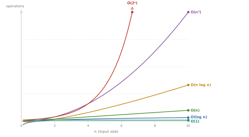
Step 4 on that list, fixing the algorithm, is usually the biggest win, because it changes which curve your program follows, not just where it sits on that curve:

Exercises

membership.py fixes target at the worst case, the last element. Measure the average case by timing lookups of many random targets, and see whether the conclusion changes.
Use timeit to find the collection size below which the list scan beats the set lookup on your machine.
Rewrite eager_first_evens() as a single list comprehension and measure its peak with tracemalloc. How close can an eager version get to the lazy one?
Apply @cache to a function that prints as a side effect, and demonstrate that repeated calls skip the printing. Explain why caching suits only pure functions.
In heap_corruption.py, replace heap.pop(0) with heappop(heap). Pop three times, printing the heap after each one, and confirm heap[0] is the smallest remaining value every time. Why does the list still look unsorted after a correct pop?
In slots.py, add class Point3D(Point) that declares no __slots__ of its own. Confirm that an instance accepts p.z = 3, which Point rejects with an AttributeError, and find where the storage for it came from.
In monitoring_counts.py, swap set_local_events() for set_events() and say which entry in the Counter is new and why. Then get the same two counts back using two local attachments instead, and explain what the two versions would stop agreeing about in a larger program.
Profile a script of your own with uv run python -m cProfile -s cumulative. Name the function with the largest tottime and the one with the largest cumtime, and explain why they are usually not the same function.
compact_array.py compares an array against a list of the same floats. Time an element-by-element sum over each with timeit. The array uses a quarter of the memory: is it also faster to iterate, and why not?
Time "".join(parts) against += in a loop for 10,000 short strings, then repeat at 100 strings. At which size does the difference stop mattering, and which of the two would you write anyway?
bisect_search.py uses bisect() and search_comparison.py uses bisect_left(). Build a sorted list with duplicates, run both against a value that appears three times, and explain which one you need to find the first occurrence and which one you need to insert after the last.
Run jit_status.py on your own interpreter and say which of the three states it reports. If it reports the second, run membership.py under PYTHON_JIT=1 and PYTHON_JIT=0 with the --numbers flag, and compare the two ratio lines. Explain why a listing this small is a poor test of the JIT.